Intro to Uber Movement Data
Authors: Alex Michels and Jinwoo Park
This notebook provides a brief overview of Uber Movement Data, demonstrates how to obtain and work with it, and illustrates a few examples of how to utilize the data for geospatial analysis.
# a few parameters/variables
FIGSIZE=(18, 12)
# import a few useful python packages
import contextily as cx
import geopandas as gpd
import pandas as pd
import matplotlib.pyplot as plt
import momepy
import osmnx as ox
import networkx as nx
import math
import numpy as np
from tqdm import tqdm
import requests
from shapely.geometry import Polygon, MultiPolygon
from shapely.errors import ShapelyDeprecationWarning
import warnings
warnings.filterwarnings("ignore", category=ShapelyDeprecationWarning) # ignore some deprecation warnings from shapely
warnings.filterwarnings("ignore", category=UserWarning) # ignore a contextily warning
Overview
Uber Movement provides access to aggregated data on travel-times, speeds, and mobility heatmaps which have been generously made available by Uber. This data is very valuable to researchers because travel-time data can be very costly to acquire. First, let's break down the three main types of data available:
- Travel-Times: This measures average travel-time (by day and time of day) between "traffic analysis zones" or neighborhoods, depending on the city. Click here for an example in London.
- Speeds: This measures the speed as a percentage of free-flow travel-time on each segment of the road. Click here for an example in New York City.
- Mobility Heatmap: This is a newer feature showing traffic density within a city. Click here for an example in Madrid.
Obtaining Uber Movement Data
While the web interface is beautiful, we need to obtain the data and combine it with other data for many of our analysis and modeling use-cases. There are two main ways to obtain the data: through the web interface and using the CLI created by Uber.
Web Interface
The web interface provides a convenient and easy way to obtain data.
First, let's visit the Uber Movement page in another tab: https://movement.uber.com/

Mouse over "Products" in the top-left corner to view the three types of data products. Let's first select "Travel Times." You should see a screen like this:

The menu on the left allows you to alterthe data by selecting date ranges, origins, and destinations. We can download the data using the "Download Data" button in the bottom-left.

The Download Data screen provides a variety of options for filtered data, all data, and geo boundaries.
Command Line Interface (CLI)
The web interface is convenient for exploring and downloading data, but there is also a Commander Line Interface (CLI) available to use called movement-data-toolkit.
Let's install the CLI:
!npm install -g movement-data-toolkit
# Let's check that the CLI installed:
# You should see the help text for the CLI print out.
!mdt --help
Using this CLI, let's download the geometry for New York in 2020:
!mdt create-geometry-file new_york 2020 > data/newyork2020.geojson
Now, we can use the Geopandas package to load the file and plot it:
df = gpd.read_file("data/newyork2020.geojson")
df.head()
# This is a rather large file and will take a minute or so to plot
df.plot(figsize=FIGSIZE)

This is great, but the geometry of the road network can be obtained elsewhere. What we really want is the speed and travel time data. The MDT CLI can also be used to get the speed data over a given date range.
The command below download the speeds in GeoJSON form New York city from November 1st, 2019 to November 2nd, 2019.
Note that it takes >10 minutes to run, so we have provided the data already and the command is commented out, but you're welcome to run the command if you're willing to wait.
If you do run the command, you can click here to skip over the very long output.
#!mdt speeds-to-geojson new_york 2019-11-01 2019-11-02 > data/nyspeed.geojson
With our data downloaded, we can load and inspect it:
speed = gpd.read_file("data/nyspeed.geojson")
speed = speed.set_crs("EPSG:4326", allow_override=True) # the CRS appears to be wrong if we don't manually set it
speed.head()
Let's plot the speed in miles per hour for each road segment:
ax = speed.plot(column="speed_mean_mph", figsize=FIGSIZE, legend=True)
cx.add_basemap(ax, crs=speed.crs.to_string(), source=cx.providers.Stamen.TonerLite)

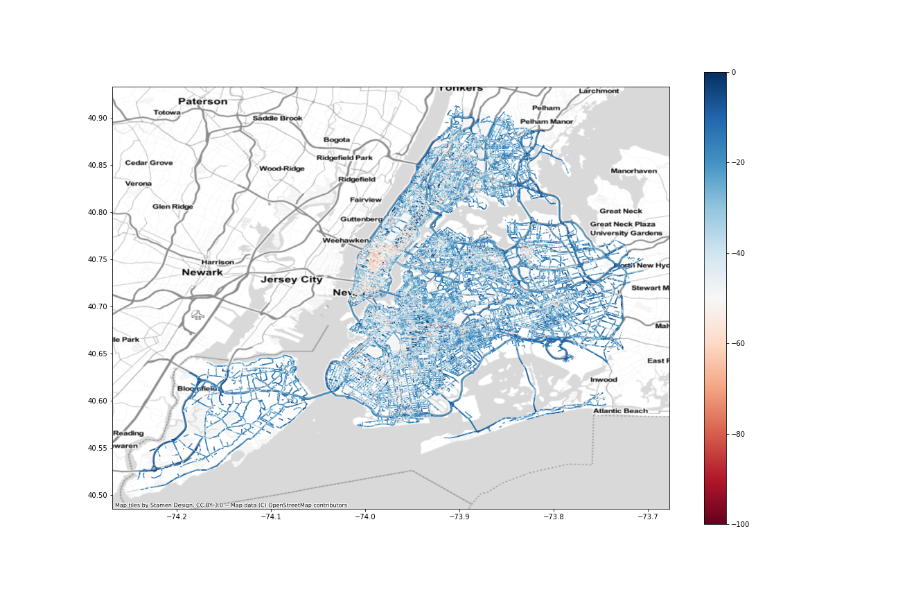
We can also plot the speed as a percentage of "free flow" which in this case means:
Free-flow speed is the term used to describe the average speed of traffic in the absence of congestion or other adverse conditions (such as bad weather). We estimate the free-flow as the 85th percentile of all speed values observed on a segment during the earliest quarter into which your filtered time range falls. In the future, we’re hoping to refine this approach and develop a more accurate representation of free-flow speeds that our users can leverage.
ax = speed.plot(column="pct_from_freeflow", figsize=FIGSIZE, cmap="RdBu", vmin=-100, vmax=0, legend=True)
cx.add_basemap(ax, crs=speed.crs.to_string(), source=cx.providers.Stamen.TonerLite)
plt.savefig("img/nyc-pct_from_freeflow.png")
plt.show()

We can theoretically create a networkx graph with the geoJSON that Uber Movements gives us, but we have run into issues in the past utilizing this graph for routing and network analysis. We have found that the better approach is to obtain our own road network from OpenStreetMap and attach the attributes we can to it.
# first, project to a non-geographic CRS like NAD83 for New York: https://epsg.io/32118
speed = speed.to_crs("EPSG:32118")
# then momepy can convert the geodataframe into a networkx graph
speednx = momepy.gdf_to_nx(speed)
type(speednx)
Uber Movement for Travel Time Calcuation
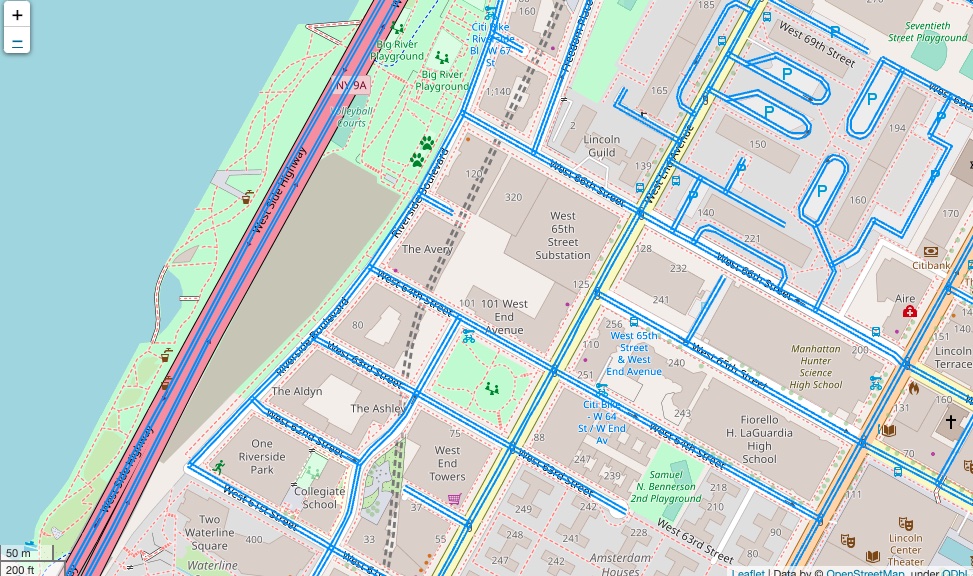
While the OSM data provided by Uber Movement is great for some purposes, it is problematic to be used for calculating travel time between two points. The figure below shows the geometry of OSM data provided by Uber. It has two edges for every road (highways on the left side), even if the road is one-way. It means that the geometry with the proper direction would have the correct travel speed data; however, the other direction of the geometry should not exist, and it would not have travel speed data, resulting in wrong free-flow traffic.
Therefore, this notebook will walk you through how to retrieve OSM data from OSM planet and integrate Uber Movement data into the OSM road network, properly.
Obtaining OpenStreetMap Data
While the Uber data is extremely useful, we also need OpenStreetMap network data (which the Uber data is based on) in network form to perform routing and network analysis. Check out our notebook if you'd like to learn more about OpenStreetmap Network data and osmnx.
Typical way using OSMnx
OSMnx provides the following functions to retrieves road network from Open Street Map.
- Getting data from an address ->
graph_from_address - Getting data from a bounding box ->
graph_from_bbox - Getting data from a geocodable place ->
graph_from_place - Getting data around some point ->
graph_from_point - Getting data for some polygon ->
graph_from_polygon
Among those five functions, we recommend to using either graph_from_place or graph_from_polygon. In this example, we demonstrate retrieving road networks using graph_from_polygon with Manhattan (New York County) geometry.
Let's obtain the driving network for Manhattan. First, we will use the census API to get the geometry for Manhattan, then pull the data from OSMNX:
# Obtain Geomery of New York County (Manhattan) from Census API.
def get_geography(geoid):
# https://api.censusreporter.org/1.0/geo/tiger2016/16000US5367000?geom=true
api_url = 'https://api.censusreporter.org/1.0/geo/latest/{0}?geom=true'
data = requests.get(api_url.format(geoid)).json()
# Get Features
fdf = pd.DataFrame({
'Geoid': geoid,
'LandArea': data['properties']['aland'] / 2589988,
'Population': data['properties']['population']
}, index=[0])
coords = data['geometry']['coordinates']
if len(coords) > 1: # If county is divided into multiple discrete parts
census_geom = MultiPolygon([Polygon(val[0]) for val in coords])
else: # If county has one contiguous geometry
census_geom = Polygon(coords[0])
fdf['geometry'] = [census_geom]
return gpd.GeoDataFrame(fdf, crs='epsg:4326', geometry = 'geometry')
# use our function to download the data and call the Geopandas `explore` function.
manhattan = get_geography('05000US36061')
manhattan.explore()
We can use this geometry to download the driving time network using the osmnx graph_from_polygon function:
# Retrieve road network within the Manhattan polygon
G = ox.graph.graph_from_polygon(manhattan['geometry'][0], network_type='drive')
ox.plot_graph(G)

Historical OSM data from OSM Planet
One critical limitation of OSMnx is that it does not support retrieving previous road networks. Given that Uber Movements data kept the OSM node and edge IDs at the time of travel, we should retrieve the road network closer to the date.
Data source
-- OSM Planet file
https://planet.openstreetmap.org/
https://ftpmirror.your.org/pub/openstreetmap/
-- Applications needed (Both programs can be installed through homebrew)
Osmosis: https://wiki.openstreetmap.org/wiki/Osmosis
Osmfilter: https://wiki.openstreetmap.org/wiki/Osmfilter
Steps to Get Historical OSM Data
Note: These steps download a large amount of data and take a long time. They are not necessary for the rest of the notebook, but explain the necessary steps to obtain historical OSM data.
- Obtain “planet-190107.osm.pbf”, replacing "190107" with the appropriate date you'd like to examine from https://ftpmirror.your.org/pub/openstreetmap/pbf/ or https://planet.openstreetmap.org/planet/full-history/
- Run the following code in the terminal to clip the original world-wide
.osm.pbf fileto the given bounding box, which is around New York City. Note:completeWays=yesandcompleteRelations=yesare important to keep the relationship after the clipping. If these two queries aren’t included,OSMnx.graph_from_xml(https://osmnx.readthedocs.io/en/stable/osmnx.html#osmnx.graph.graph_from_xml) will return error.
osmosis \
--read-pbf planet-190107.osm.pbf \
--bounding-box top=40.917705 \
left=-74.358714 \
bottom=40.491167 \
right=-73.700169 \
completeWays=yes \
completeRelations=yes \
--write-xml planet_190107_nyc.osm- Query only the road network that car can travel. The criteria is as below based on the ones provided by OSMnx.
- Use
osmfilterin the terminal to select edges with highway tag.
Note:osmfilteris used for this process sinceosmosissayshighway=*is not found although its documentation says it is possible.
osmfilter planet_190107_nyc.osm \
--keep="highway=" \
-o=nyc_190107_all_highways.osm- After selecting every edge with highway tag, we want to remove edges with tags indicating cars cannot travel on their edges. Run the following code on the terminal.
osmosis \
--read-xml nyc_190107_all_highways.osm \
--tf reject-ways highway=abandoned,bus_guideway,construction,corridor,cycleway,elevator,escalator,footway,path,pedestrian,planned,platform,proposed,raceway,service,steps \
--tf reject-ways access=private \
--tf reject-ways motor_vehicle=no \
--tf reject-ways motorcar=no \
--tf reject-ways service=alley,driveway,emergency_access,parking,parking_aisle,private\
--tf reject-relations\
--used-node \
--write-xml nyc_190107_cleaned.osm- RESULTED FILE (
*.osm) can be imported to OSMnx withox.graph_from_xml()function and then it can be exported to*.graphmlfile.
# Load Historical OSM network obtained from OSM Planet
G = ox.load_graphml('./data/manhattan_network.graphml')
ox.plot_graph(G)

Preprocessing Road Network
This step preprocesses the road network from Open Street Map to make it ready to merge with Uber Movement data. Given that OSM is crowd-sourced datasets, it sometimes possesses issues preventing effective integration, such as disconnected networks and lack of speed limit information.
First, we will define a function to remove nodes that you can't travel from:
def remove_unnecessary_nodes(network):
"""
Removes nodes with no outdegree (nodes you cannot "leave").
Args:
network - networkx.classes.multidigraph.MultiDiGraph
Returns:
networkx.classes.multidigraph.MultiDiGraph - network with nodes removed.
"""
_nodes_removed = len([n for (n, deg) in network.out_degree() if deg == 0])
network.remove_nodes_from([n for (n, deg) in network.out_degree() if deg == 0])
for component in list(nx.strongly_connected_components(network)):
if len(component) < 100:
for node in component:
_nodes_removed += 1
network.remove_node(node)
print("Removed {} nodes ({:2.4f}%) from the OSMNX network".format(_nodes_removed, _nodes_removed / float(
network.number_of_nodes())))
print("Number of nodes: {}".format(network.number_of_nodes()))
print("Number of edges: {}".format(network.number_of_edges()))
return network
Next, we will remove any edges of the graph that do not support road travel:
def remove_unnecessary_edges(network, road_types):
"""
Remove edges that car cannot travel; retrieved based on 'highway' attribute
Args:
network - networkx.classes.multidigraph.MultiDiGraph
road_types - List[str], way types to remove
Returns:
networkx.classes.multidigraph.MultiDiGraph - network with ways removed.
"""
_edges_removed = 0
for u, v, data in network.copy().edges(data=True):
if 'highway' in data.keys():
if type(data['highway']) == list:
highway_type = data['highway'][0]
else:
highway_type = data['highway']
if highway_type in road_types: # Car cannot travel on these types of road
network.remove_edge(u, v)
_edges_removed += 1
print("Removed {} edges ({:2.4f}%) from the OSMNX network".format(_edges_removed, _edges_removed /
float(network.number_of_edges())))
return network
Now, we can apply these two functions to our road network:
# Remove disconnected network and unnecessary road types (e.g., bridleway)
G = remove_unnecessary_edges(G, ['bridleway', 'access'])
G = remove_unnecessary_nodes(G)
Now, we want to assign the usual maximum speeds to roads where we do not have information based on the type of the roadway:
def assign_max_speed_with_highway_type(network):
"""
Assigns the speed limit to each way based on the way type. Maxspeed here was obtained from the mode
of `maxspeed` attribute per `highway` type.
Args:
network - networkx.classes.multidigraph.MultiDiGraph
Returns:
networkx.classes.multidigraph.MultiDiGraph, with speed limits added
"""
max_speed_per_type = {'motorway': 50,
'motorway_link': 30,
'trunk': 35,
'trunk_link': 25,
'primary': 25,
'primary_link': 25,
'secondary': 25,
'secondary_link': 25,
'tertiary': 25,
'tertiary_link': 25,
'residential': 25,
'living_street': 25,
'unclassified': 25,
'road': 25,
'track': 25
}
for u, v, data in network.edges(data=True):
# Assign the maximum speed of edges based on either 'maxspeed' or 'highway' attributes
if 'maxspeed' in data.keys():
if type(data['maxspeed']) == list:
temp_speed = data['maxspeed'][0] # extract only the first entry if there are many
else:
temp_speed = data['maxspeed']
if type(temp_speed) == str:
temp_speed = temp_speed.split(' ')[0] # Extract only the number
temp_speed = int(temp_speed)
else:
if 'highway' in data.keys():
# if the variable is a list, grab just the first one.
if type(data['highway']) == list:
road_type = data['highway'][0]
else:
road_type = data['highway']
# If the maximum speed of the road_type is predefined.
if road_type in max_speed_per_type.keys():
temp_speed = max_speed_per_type[road_type]
else: # If not defined, just use 20 mph.
temp_speed = 20
else:
temp_speed = 20
data['maxspeed'] = temp_speed # Assign back to the original entry
return network
# Apply the function
G = assign_max_speed_with_highway_type(G)
Converting our network back to a GeoDataFrame can be easily achieved using the osmnx graph_to_gdfs function.
nodes, edges = ox.graph_to_gdfs(G, nodes=True, edges=True, node_geometry=True)
edges.head()
Using Uber Movement Data
Approach 1: Match based on the start and end node IDs
Uber movements data provides each hour's time-dependent travel speed as average (speed_mph_mean) and standard deviation (speed_mph_stddev). Each hour record has osm_way_id, osm_start_node_id, and osm_end_node_id.
In this step, we match the uber movement data with OSM based on the start and end node IDs.
The sample data (uber_df) has the traffic speed of roads in Manhattan, New York City, for 12 o'clock between May 6, 2019 and May 10, 2019.
uber_df = pd.read_csv('./data/uber_may_second_week_noon.csv')
uber_df.head(3)
def calculate_weighted_mean(means, stds):
"""
Calculates the inverse-standard deviation weighted mean.
Args:
means - List[float], the means
stds - List[float], the standard deviations
Returns:
the inverse-standard deviation weighted mean
"""
return sum(means * 1 / stds) / sum(1 / stds)
def join_uber_data_with_osm_edges_(network, uber_hour_df):
"""
Assigns the inverse-standard deviation weighted mean of uber speeds to the network for matching ways.
Args:
network - networkx.classes.multidigraph.MultiDiGraph
uber_hour_df - pandas.DataFrame of ways
Returns:
networkx.classes.multidigraph.MultiDiGraph with weighted mean travel-time added.
"""
for u, v, data in tqdm(network.edges(data=True)):
# When travel time records in uber dataset match with OSM based on origin (u) and destination (v),
# we update `uber_speed` of network (G) based on the uber records.
match_ori_dest = uber_hour_df.loc[(uber_hour_df['osm_start_node_id'] == u) &
(uber_hour_df['osm_end_node_id'] == v)
]
# If there are matching records,
# we average the travel time of Uber with the inverse weights of standard deviation.
# Higher standard deviation has less weight
if match_ori_dest.shape[0] > 0:
weighted_mean = calculate_weighted_mean(match_ori_dest['speed_mph_mean'].values,
match_ori_dest['speed_mph_stddev'].values
)
data['uber_speed'] = weighted_mean
# If there is no matching records based on the origin (u) and destination (v),
# we just skip the corresponding row for now.
else:
pass
return network
Run the above function to add the speed data:
G_ = join_uber_data_with_osm_edges_(G, uber_df)
Now, we can export the graph data to a GeoDataFrame for easy statistics, inspection, and visualization. We will also calculate speed_ratio as the ratio between the uber speed and the maximum speed limit on the road segment:
# Export NetworkX to GeoDataFrame for Visualization
nodes_, edges_ = ox.graph_to_gdfs(G_, nodes=True, edges=True, node_geometry=True)
# Calculate the ratio of edges that don't have travel speed provided by Uber Movement.
ratio_ = edges_.loc[~edges_['uber_speed'].isna()].shape[0] / edges_.shape[0]
print(f"{round(ratio_, 3) * 100}% of edges have recorded travel speed.")
edges_['speed_ratio'] = edges_.apply(lambda x:x['uber_speed'] / x['maxspeed'], axis=1)
edges_.head()
Let's plot the Uber speed data (left) and the speed as a function of the maximum speed for each road segment:
fig, axes = plt.subplots(1,2, figsize=(15, 10))
edges_.loc[edges_['uber_speed'].isna()].plot(color='black', ax=axes[0], linewidth=0.5)
edges_.plot('uber_speed', ax=axes[0], cmap='Blues', legend=True)
edges_.loc[edges_['uber_speed'].isna()].plot(color='black', ax=axes[1], linewidth=0.5)
edges_.plot('speed_ratio', ax=axes[1], cmap='RdBu', vmin=0 , vmax=1 ,legend=True)

Approach 2: Match with Edge ID and Azimuth of edges
Given that the matching rate with start and end nodes IDs was not successful, we here try to bring OSM ids for edges. But, in the meantime, we also should be cautious about matching the wrong travel speed with the wrong edges. Therefore, I integrated a step for checking the azimuth of edges, comparing it with the osm dataset provided by Uber.
This step assumes a case that the edge IDs remain the same, but node IDs have updated.
# Import OSM data provided by Uber
uber_osm = gpd.read_file('./data/newyork2020.geojson')
uber_osm = uber_osm.set_crs(epsg=4326, allow_override=True)
Let's investigate the road network (OSM) geometry retrieved from OSM Planet and Uber Movement.
The two maps at the bottom describe the geometry of the same road. But OSM Planet data has it as a single geometry, while Uber Movement/OSM has two lines, indicating both directions.
fig, axes = plt.subplots(2, 1, figsize=(10, 10))
edges.loc[edges['osmid'] == 44164416].plot(ax=axes[0])
cx.add_basemap(axes[0], crs=uber_osm.crs.to_string())
axes[0].set_title('OSM data from OSMnx/OSM Planet', fontsize=15)
uber_osm.loc[uber_osm['osmwayid'] == 44164416].plot(ax=axes[1])
cx.add_basemap(axes[1], crs=uber_osm.crs.to_string())
axes[1].set_title('OSM data from Uber Movement', fontsize=15)
axes[0].get_xaxis().set_visible(False)
axes[0].get_yaxis().set_visible(False)
axes[1].get_xaxis().set_visible(False)
axes[1].get_yaxis().set_visible(False)
fig.tight_layout()

def calculate_azimuth(x1, y1, x2, y2):
# Calculate the azimuth between two points
d_x = x2 - x1 # Delta of x coordinates
d_y = y2 - y1 # Delta of y coordinates
temp_azimuth = math.degrees(math.atan2(d_x, d_y)) # Calculate Azimuth from the ArcTangent of two delta values.
if temp_azimuth > 0:
return temp_azimuth
else:
return temp_azimuth + 360
def assign_speed_based_on_azimuth(network, u, v, match_df, uber_osm_edges):
# The azimuth of current edges in the loop
current_azimuth = round(calculate_azimuth(network.nodes[u]['x'], network.nodes[u]['y'],
network.nodes[v]['x'], network.nodes[v]['y']), -1)
match_df = match_df.merge(uber_osm_edges,
left_on=['osm_start_node_id', 'osm_end_node_id'],
right_on=['osmstartnodeid', 'osmendnodeid']
)
if match_df.shape[0] > 0:
match_df['azimuth'] = match_df.apply(lambda x: round(calculate_azimuth(x.geometry.coords[:][0][0],
x.geometry.coords[:][0][1],
x.geometry.coords[:][-1][0],
x.geometry.coords[:][-1][1]),
-1),
axis=1)
# Consider two edges are the same,
# if the azimuth of the current edges are within += 10 degree compared to the uber osm data.
edges_of_interest = match_df.loc[match_df['azimuth'].isin([i + current_azimuth for i in range(-30, 40, 10)])]
if edges_of_interest.shape[0] > 0:
return calculate_weighted_mean(edges_of_interest['speed_mph_mean'], edges_of_interest['speed_mph_stddev'])
else:
return np.nan
else:
return np.nan
def join_uber_data_with_osm_edges(network, uber_hour_df, uber_osm_gdf):
# Tries to match the Uber and OSM data using IDs and azimuth
for u, v, data in tqdm(network.edges(data=True)):
# When travel time records in uber dataset match with OSM based on origin (u) and destination (v),
# we update `uber_speed` of network (G) based on the uber records.
match_ori_dest = uber_hour_df.loc[(uber_hour_df['osm_start_node_id'] == u) &
(uber_hour_df['osm_end_node_id'] == v)]
# If there are matching records,
# we average the travel time of Uber with the inverse weights of standard deviation.
# Higher standard deviation has less weight
if match_ori_dest.shape[0] > 0:
weighted_mean = calculate_weighted_mean(match_ori_dest['speed_mph_mean'].values,
match_ori_dest['speed_mph_stddev'].values)
data['uber_speed'] = weighted_mean
# If there is no matching records based on the origin (u) and destination (v),
# we now try to match with their osm_way_id.
# Given the osm_way_id is assigned based on the road names (i.e., multiple edges per osm_way_id),
# we need to match the direction of edges (based on azimuth of edges) to retrieve travel time properly.
else:
if type(data['osmid']) == int:
match_osmid = uber_hour_df.loc[uber_hour_df['osm_way_id'] == data['osmid']]
if match_osmid.shape[0] > 0:
weighted_mean = assign_speed_based_on_azimuth(network, u, v, match_osmid, uber_osm_gdf)
data['uber_speed'] = weighted_mean
elif type(data['osmid']) == list:
speed_list = []
for temp_id in data['osmid']:
match_osmid = uber_hour_df.loc[uber_hour_df['osm_way_id'] == temp_id]
if match_osmid.shape[0] > 0:
weighted_mean = assign_speed_based_on_azimuth(network, u, v, match_osmid, uber_osm_gdf)
speed_list.append(weighted_mean)
if speed_list:
data['uber_speed'] = sum(speed_list) / len(speed_list)
return network
G = join_uber_data_with_osm_edges(G, uber_df, uber_osm)
With the data matched, we can export NetworkX to GeoDataFrame for Visualization:
nodes, edges = ox.graph_to_gdfs(G, nodes=True, edges=True, node_geometry=True)
# Calculate the ratio of edges that don't have travel speed provided by Uber Movement.
ratio = edges.loc[~edges['uber_speed'].isna()].shape[0] / edges_.shape[0]
print(f"{round(ratio, 3) * 100}% of edges have recorded travel speed.")
edges['speed_ratio'] = edges.apply(lambda x:x['uber_speed'] / x['maxspeed'], axis=1)
edges.loc[edges['osmid'] == 44164416].sort_values(by='length')
fig, axes = plt.subplots(1,2, figsize=(15, 10))
edges.loc[edges['uber_speed'].isna()].plot(color='black', ax=axes[0], linewidth=0.5)
edges.plot('uber_speed', ax=axes[0], cmap='Blues', legend=True)
edges.loc[edges['uber_speed'].isna()].plot(color='black', ax=axes[1], linewidth=0.5)
edges.plot('speed_ratio', ax=axes[1], cmap='RdBu', vmin=0 , vmax=1 ,legend=True)

Learn More / References
Blogs and Informal Resources
Academic Papers
- Boeing, Geoff. "OSMnx: New methods for acquiring, constructing, analyzing, and visualizing complex street networks" https://doi.org/10.1016/j.compenvurbsys.2017.05.004