PRIME: A CyberGIS Platform for Resilience Inference Measurement and Enhancement

Authors : Debayan Mandal 1, Dr. Lei Zou1,*, Rohan Singh Wilkho3, Joynal Abedin1, Bing Zhou1, Dr. Heng Cai2, Dr. Furqan Baig4, Dr. Nasir Gharaibeh3, Dr. Nina Lam5

1 Geospatial Exploration and Resolution (GEAR) Lab, Department of Geography, College of Geosciences, Texas A & M University
2 GIResilience Lab, Department of Geography, College of Geosciences, Texas A & M University
3 Zachry Department of Civil and Environmental Engineering, College of Engineering, Texas A & M University
4 CyberGIS Center for Advanced Digital & Spatial Studies, University of Illinois at Urbana-Champaign
5 Department of Environmental Sciences, College of the Coast & Environment, Louisiana State University
* Corresponding author: lzou@tamu.edu

You can checkout the paper here: https://doi.org/10.48550/arXiv.2404.09463


Introduction

Resilience assessment and improvement have become increasingly important in today's world, where natural and man-made disasters are becoming more frequent and severe. Cities, communities, and organizations are recognizing the need to prepare for and mitigate the impacts of disasters and disruptions, and there is a growing body of research and practice on resilience assessment and improvement.

One significant research gap in this area is the lack of a customizable platform for resilience assessment and improvement. While there are many tools and frameworks available for assessing and improving resilience, they are often limited in their scope and applicability. Many of these tools are designed for specific types of hazards or sectors and may not be easily adapted to other contexts. Furthermore, many of these tools are proprietary and require significant resources to implement and maintain.

A customizable platform for resilience assessment and improvement would address these limitations by providing a flexible and adaptable framework that can be tailored to the needs and priorities of different users. Such a platform would allow users to customize the tools and metrics used for resilience assessment, as well as the interventions and strategies for resilience improvement. This would enable users to address specific challenges and opportunities in their context, and to leverage existing resources and knowledge to support resilience. By enabling users to tailor resilience assessment and improvement to their specific needs and priorities, such a platform would help to build more resilient communities, organizations, and systems, and contribute to a more sustainable and resilient future for all.

Resilience Inference Measurement Model

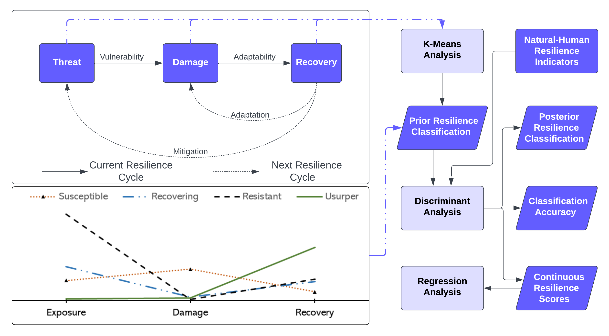
The Resilience Inference Measurement (RIM) model was developed by Dr. Nina Lam to measure disaster resilience of various units of the community, viz. individuals and organizations. It is based on the idea that resilience is dependent on adaptability as well as vulnerability, i.e., not just the ability to bounce back from adversity, but also the ability to adapt and thrive in the face of ongoing challenges and stressors. The RIM model is unique in that it evaluates resilience using empirical disaster measures such as threat, damage and recovery in line with the Sendai Framework, as well as taking on a holistic approach to measuring resilience, incorporating not only empirical factors but also the broader social and environmental context. This makes it a powerful tool for identifying areas of strength and weakness in resilience and for developing targeted interventions and strategies to build resilience in communities.
Image

The above figure suggests the preliminary idea that in one resilience cycle vulnerability is dependent on exposure and damage, while adaptability is dependent upon the damage and recovery from the natural hazard. This goes into a feedback loop and updates itself in the next resilience cycle where mitigation procedures from recovery activities reduce exposure to the particular disaster while adaptation measures reduce future disaster damages.

Enhanced Customizable Framework

Image

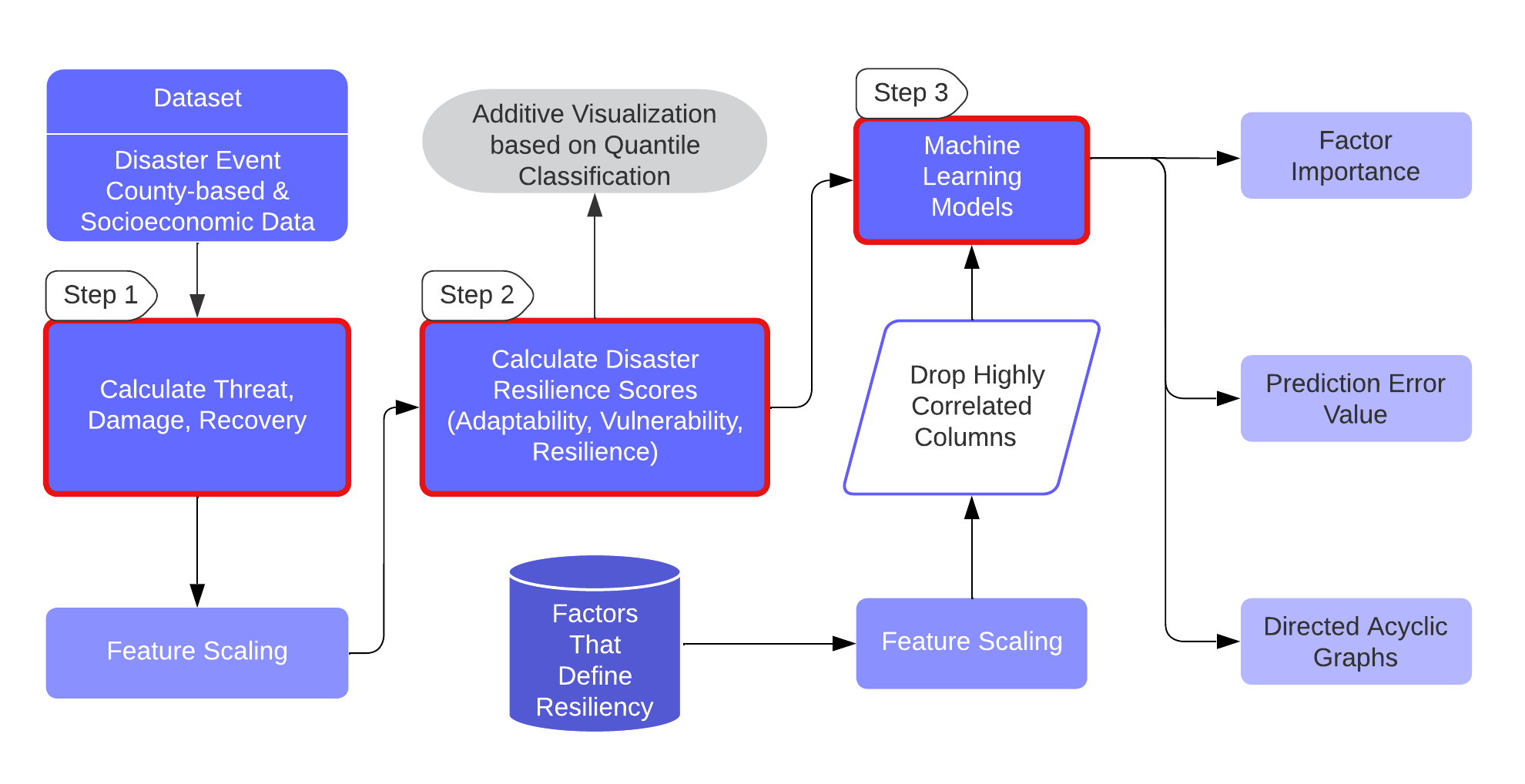
In formulating the CRIM model, we have based it on the fundamental framework of the RIM and addressed its limitations. Please refer to our paper for detailed breakdown of the enhancements and customizations. The workflow mainly operates using disaster event and socioeconomic datasets. In Step 1 and 2, it calculates resilience scores (adaptability, vulnerability, resilience) based on empirical parameters of hazard threat, damage, and recovery. In Step 3, CRIM uses machine learning regressors to learn the relationships between the resultant scores and socio-economic factors characterizing a community. These relationships are validated using a held-out test dataset. This not only confirms the reliability of the identified relationships but also ensures their generalizability.

Prerequisites to Model Implementation

This code has been tested to run properly for Python 3-0.9.0. Please make sure to choose that kernel so as not to run into any errors.

In [1]:
import warnings
from sklearn.preprocessing import MinMaxScaler
warnings.filterwarnings("ignore")
In [2]:
!pip install xgboost --quiet

All the Inputs

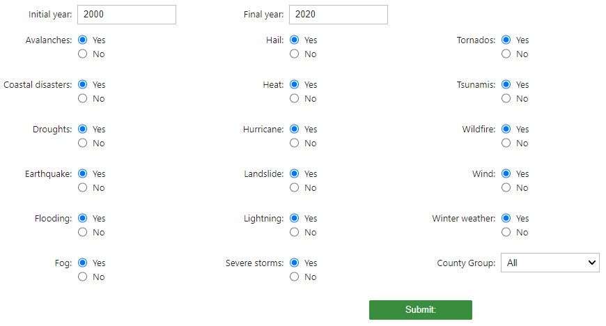
This section is only for entering filtering parameters from the whole dataset
Sample:
Image
In [3]:
import preprocess as prep
widget_dict = prep.create_gui1()
In [4]:
prep.print1(widget_dict)
The inputted parameters are:
Duration to be computed:2000 to 2020 

The hazards considered in this computation are:
Avalanche, Tornado, Coastal, Flooding, SevereStorm, Wind, Drought, Heat, Earthquake, Fog, WinterWeather, Hail, Landslide, Lightning, Tsunami, Wildfire, Hurricane

All counties will be evaluated

Data Pre-processing

In [5]:
fn = prep.process_data(widget_dict)

Three Empirical Factor Calculation

Image

To realize these frameworks, we incorporated formulas aimed at quantifying the otherwise abstract concepts of vulnerability and adaptability. In the CRIM framework, we first compute the three empirical parameters: threat, damage, and recovery using the Comprehensive Hazard and Population data per year.

Threat (per hazard event) = Duration(days) * Likelihood * Weightage

(Equation 1)

Likelihood (per hazard type) = Count / Total Days

(Equation 2)

Weight (per hazard type) = Mean Damage per day per capita

(Equation 3)


Damage per capita (per hazard event) = (Crop Damage + Property Damage) / Initial Population

(Equation 4)


Recovery Rate (per county) = (Final Population - Initial Population) / Initial Population

(Equation 5)


These equations are entirely modifiable as per requirements of the study


Equation 1:
The first component, duration, refers to the length of the historic hazard events, expressed in days. This variable recognizes that the impact of a hazard event typically increases with its duration. The second component is the likelihood, which quantifies the probability frequency distribution of hazard type per day (Equation 2). This factor acknowledges the inherent uncertainty in the occurrence of hazard events. The third component is the weight for each hazard event type. This weightage of each hazard event type is depicted as the mean damage caused per day per capita in a county. This factor recognizes that different hazard types can have different impacts based on its nature. For example, tornadoes might occur more frequently but cause less average damage than earthquakes. To calculate the weight (Equation 3), we assessed the individual damage data for each event to determine the mean damage per day per capita for each hazard event type.

Equation 4:
We derive a per capita estimate of the damage by dividing the sum of these damages by the pre-event initial population. Crop damage refers to the harm inflicted on agricultural produce by the disaster, which can impact local economies, particularly in areas heavily dependent on agriculture. Property damage pertains to the destruction of infrastructure (homes, businesses, public facilities) which has direct and immediate impact on urban residents' living conditions and livelihoods.

Equation 5:
the recovery variable gives a quantification of the community trying to return back to its original state before disaster. As population change is one prominent factor for quantifying how the community works despite disaster, i.e., if there has been migration to and from the community - this has been chosen as a Recovery factor. The increase in population has been calculated to be the recovery factor. A higher recovery rate for a county signifies an increase in population after the disaster events, indicating successful society rebuilding efforts.

In [6]:
edr_tot = prep.empfac(fn, widget_dict)

Disaster Resilience Indexes

Image

Finally, the resilience indexes are calculated. The calculations and concepts are discussed in the following sections. For normalization technique we have opted for minmax scaling. MinMax Scaling rescales numeric features into a common range, typically 0 to 1, ensuring that no particular feature dominates due to its numeric range. The calculation involves subtracting the minimum value of a feature, then dividing by its range (maximum - minimum). This technique maintains the original distribution's shape but doesn't handle outliers well. In the new scale, the minimum value becomes 0, the maximum 1, and all other values fall proportionally within this range. It is particularly beneficial when the data does not follow a Gaussian distribution, which was the case with several of our parameters.
Users may modify the code to opt for z-score normalization too if the data follows a Gaussian distribution

Adaptability Calculation

Adaptability in disaster resilience refers to the ability of a community or system to adjust and respond effectively to changes or disruptions caused by a disaster. This includes the capacity to anticipate, absorb, and recover from the impacts of a disaster, and to learn from the experience in order to better prepare for future events. It is quantified using the Equation 6. Here, the difference is obtained after normalization as both the minuend and subtrahends are of different units.

Adaptability = Normalized Recovery – Normalized Damage

(Equation 6)

Vulnerability Calculation

Vulnerability in disaster resilience refers to the susceptibility of a community or system to potential harm or damage caused by natural or human-made hazards. This can be influenced by various factors such as socioeconomic status, physical and environmental conditions, and access to resources and services. Reducing vulnerability is a crucial aspect of building resilience to disasters, as it enables communities to better withstand and recover from the impacts of disasters. We compute vulnerability as the normalized differential between damage and threat (equation 7). We express both these factors in the same units, and hence, obtain the difference before normalizing. The underlying principle contends that a community enduring equivalent destruction from infrequent disasters would be perceived as more vulnerable compared to a community exposed to more recurrent disasters.

Vulnerability = Normalized Damage – Normalized Threat

(Equation 7)

Resilience Calculation

Resilience Score (equation 8) is a comprehensive measure of a community’s resilience to disasters. We interpret it as the relation between the adaptability and vulnerability of a community, and it is formulated as follows:

Resilience = Adaptability – Vulnerability

(Equation 8)

It implies that increasing a community's adaptability or reducing its vulnerability would improve the community's overall resilience score to disasters. These thus offer us insights into the dynamics of disaster impact and recovery.

In [7]:
edr_tot,prgr = prep.disres(edr_tot)

Priori Group Visualization

Image

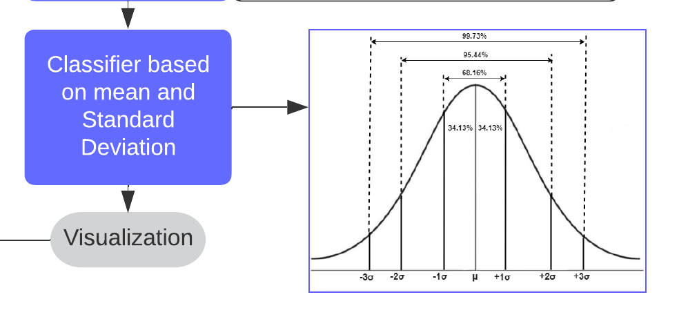
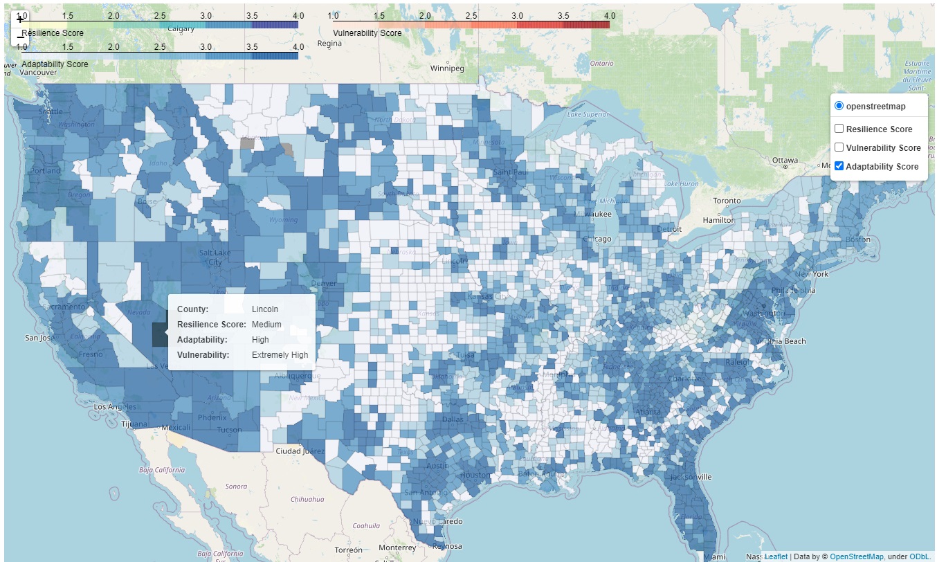
For exploratory analysis purposes, we propose that the resultant scores are additive in nature. Under this assumption, we suggest that long-term resilience over the whole study period could be understood as the average of their yearly counterparts. It is a simplified perspective intended to provide an overarching view of the community's disaster resilience over a longer span. A quantile classification function in incorporated that transforms the continuous scores into four categories. This interactive map interface visualizes these resilience, vulnerability, and adaptability categories, in different choropleth layers, across different counties.

Sample:
Image
In [8]:
final_df = prep.gencpleth(prgr, "data/counties/geojson-counties-fips.json", widget_dict['ini'].value, widget_dict['fin'].value)

This displays the aggregate resilience indexes from 2000 to 2020

Make this Notebook Trusted to load map: File -> Trust Notebook

Socio-Economic Data Processing

Post Groups with Customisable Machine Learning

Image

Our framework integrates a selection of machine learning models, covering both white-box (fully interpretable) and grey-box (partially interpretable) regressor models. These models are applied to validate the resilience scores obtained in relation to socioeconomic factors and develop a predictive model. The framework computes performance error metrics dependent upon the choice of regressors. Ultimately, the choice of the most precise model for such predictive tasks is left to the users. To provide explainability, the framework depicts the relationship between the socio-economic variables and resilience scores using coefficients, importance scores, and directed arcs.

Our process for each model follows the sequence of hyperparameter tuning, re-training tuned models and model evaluation. We optimize model performance through hyperparameter tuning, selecting models yielding the lowest MAE values in the cross-validation process. After determining the optimized hyperparameters, we initialize the models with these parameters and re-train them on the original training set. Subsequently, we assess the model performance by computing evaluation metrics on the held-out testing set.

Variable Correlation

Checking data correlation:

Sample:

Image
In [9]:
import corr as corr
X, data, corr_matrix = corr.matrix('data/variables', widget_dict['ini'].value, widget_dict['fin'].value, final_df)

In general, it is desirable to avoid using highly correlated independent variables as inputs to a machine learning model. This is because highly correlated variables can lead to overfitting, where the model fits the noise in the data instead of the underlying relationships between the independent and dependent variables. A commonly used rule of thumb is to avoid using variables with a correlation coefficient above 0.7 or below -0.7. However, the exact threshold for acceptable correlation depends on the specific problem and the nature of the data. It is generally a good idea to examine the pairwise correlation between the independent variables and remove highly correlated variables before fitting a machine learning model.

Sample:

Image
In [10]:
choice = corr.remopt()
Enter method for dropping columns: 
In [11]:
columns_to_drop = corr.optionA(data) if choice.value == 'Remove by selecting names' else corr.optionB(data) if choice.value == 'Remove by correlation index' else None
Columns being removed because of high correlation:

Households with atleast 1 vehicle
General Medical And Surgical Hospitals
Household with no plumbing
Emergency Services Personnel
Living Alone
Geographical Mobility Same House 1 Year Ago
Median Household Income

Please press Enter after inputting the desired correlation index if the second option is chosen

In [12]:
X = corr.dropcol(X, columns_to_drop)
In [13]:
save_df,X = corr.makedf(X, prgr)
Number of entries with no value: 14655

Feature Scaling

This is done to have an unbiased evaluation. Otherwise Eucledian distance mire the results. If the features are on different scales, the larger ones can have a disproportionately large effect on the model, leading to biased results. By scaling the features to have zero mean and unit variance (using techniques such as StandardScaler or MinMaxScaler), we can ensure that all independent features have a similar impact on the model.

In [14]:
X = MinMaxScaler().fit_transform(X)

Test-train split

It divides the entire dataset into a user-inputted split. The training set is used to perform training and hyperparameter tuning, and the testing set to compare the tuned models’ performances. Please click "Submit" after entering the parameters. The input will also be printed in the console log for verification if needed.

Sample:

Image
In [15]:
import ML
test_split, random_state = ML.split()
In [16]:
splits = ML.split_data(X, save_df['Y_Class'], save_df['YV_Class'], save_df['YA_Class'], save_df['YV_Value'], save_df['YA_Value'], save_df['YR_Value'], test_split, random_state)

Regressors

Linear Regression

Linear regression is a statistical method used to study the relationship between two continuous variables by fitting a linear equation to the observed data. The goal of linear regression is to find the best-fit line that can predict the value of the dependent variable (Y) based on the value of the independent variable (X).

Pros:

  • Simple and easy to understand.
  • Fast and computationally efficient.
  • Works well when the relationship between variables is linear.

Cons:

  • Assumes a linear relationship between variables, which may not always hold true.
  • Sensitive to outliers, as they can significantly impact the fit of the model.
  • Cannot handle non-linear relationships or interactions between variables.

Adaptability

In [17]:
best_model, feature_importance_df = ML.perform_linear_regression(splits, 'Xar_train', 'yar_train', 'Xar_test', 'yar_test', save_df)
MSE: 0.00034
RMSE: 0.01846
MAE: 0.00692

For higher degree polynomial fitting:

In [19]:
best_model, feature_importance_df = ML.perform_poly_regression(splits, 'Xar_train', 'yar_train', 'Xar_test', 'yar_test', save_df, range(1, 3))
Best Degree: 1
Minimum MSE: 0.00034
MSE: 0.00034
RMSE: 0.01846
MAE: 0.00652

Vulnerability

In [20]:
best_model, feature_importance_df = ML.perform_linear_regression(splits, 'Xvr_train', 'yvr_train', 'Xvr_test', 'yvr_test', save_df)
MSE: 0.00016
RMSE: 0.01252
MAE: 0.00176

For higher degree polynomial fitting:

In [21]:
best_model, feature_importance_df = ML.perform_poly_regression(splits, 'Xvr_train', 'yvr_train', 'Xvr_test', 'yvr_test', save_df, range(1, 3))
Best Degree: 1
Minimum MSE: 0.00016
MSE: 0.00016
RMSE: 0.01252
MAE: 0.00183

Resilience

In [22]:
best_model, feature_importance_df = ML.perform_linear_regression(splits, 'Xrr_train', 'yrr_train', 'Xrr_test', 'yrr_test', save_df)
MSE: 0.00052
RMSE: 0.02278
MAE: 0.00530

For higher degree polynomial fitting:

In [23]:
best_model, feature_importance_df = ML.perform_poly_regression(splits, 'Xrr_train', 'yrr_train', 'Xrr_test', 'yrr_test', save_df, range(1, 3))
Best Degree: 1
Minimum MSE: 0.00052
MSE: 0.00052
RMSE: 0.02278
MAE: 0.00508

Ridge Regression

Ridge regression is a linear regression algorithm used to deal with multicollinearity in data. It adds a penalty term to the sum of squared errors that forces the model to choose smaller coefficients for correlated variables. This helps to reduce the variance in the model by shrinking the regression coefficients towards zero.

Pros of Ridge Regression:

  • Helps to deal with multicollinearity in the data
  • Can improve the stability and generalization performance of the model
  • Can prevent overfitting of the model by reducing the variance in the estimates
  • Works well when the number of predictors is larger than the number of samples

Cons of Ridge Regression:

  • The selection of the penalty parameter is crucial for the performance of the model
  • It assumes that all predictors are relevant to the outcome, which may not always be the case
  • It does not perform feature selection, meaning all variables will be retained in the model, which can lead to overfitting

Adaptability

In [24]:
best_model, importances = ML.perform_ridge_regression(splits, 'Xar_train', 'yar_train', 'Xar_test', 'yar_test', save_df)
MSE: 0.00034
RMSE: 0.01846
MAE: 0.00692

Vulnerability

In [25]:
best_model, importances = ML.perform_ridge_regression(splits, 'Xvr_train', 'yvr_train', 'Xvr_test', 'yvr_test', save_df)
MSE: 0.00016
RMSE: 0.01252
MAE: 0.00176

Resilience

In [26]:
best_model, importances = ML.perform_ridge_regression(splits, 'Xrr_train', 'yrr_train', 'Xrr_test', 'yrr_test', save_df)
MSE: 0.00052
RMSE: 0.02278
MAE: 0.00529

Support Vector Regression

Adaptability

In [ ]:
best_model, importances = ML.perform_svr(splits, 'Xar_train', 'yar_train', 'Xar_test', 'yar_test', save_df)

Vulnerability

In [ ]:
best_model, importances = ML.perform_svr(splits, 'Xvr_train', 'yvr_train', 'Xvr_test', 'yvr_test', save_df)

Resilience

In [ ]:
best_model, importances = ML.perform_svr(splits, 'Xrr_train', 'yrr_train', 'Xrr_test', 'yrr_test', save_df)

Random Forest Regression

Random Forest Regression builds a number of decision trees on a randomly selected subset of the training set, and then averages the predictions of each tree to produce the final prediction. The randomness in the selection of features and samples reduces the variance and overfitting.

Pros:

  • Handles high dimensional datasets well
  • Can handle both categorical and continuous data
  • Tends to have good predictive accuracy
  • Provides a measure of feature importance

Cons:

  • Can be slower than other regression algorithms due to the large number of trees
  • Can be difficult to interpret the relationships between the independent and dependent variables
  • May overfit the training data if the number of trees is too large

Adaptability

In [27]:
best_model, importances = ML.perform_random_forest(splits, 'Xar_train', 'yar_train', 'Xar_test', 'yar_test', save_df, random_state)
MSE: 0.0003194777055431521
RMSE: 0.017873939284420548
MAE: 0.005748392591169003

Vulnerability

In [28]:
best_model, importances = ML.perform_random_forest(splits, 'Xvr_train', 'yvr_train', 'Xvr_test', 'yvr_test', save_df, random_state)
MSE: 0.00015487748787118143
RMSE: 0.012444978419876084
MAE: 0.0017970720583366875

Resilience

In [29]:
best_model, importances = ML.perform_random_forest(splits, 'Xrr_train', 'yrr_train', 'Xrr_test', 'yrr_test', save_df, random_state)
MSE: 0.0005067027843961834
RMSE: 0.02251005962666877
MAE: 0.004664485230912826

XGBoost Regression

XGBoost Regression is a type of regression algorithm that uses an ensemble of decision trees to make predictions. It is an extension of the gradient boosting algorithm, and is known for its high predictive power and speed.

Pros:

  • High accuracy: XGBoost Regression is known for its high accuracy and predictive power, making it a popular choice for regression tasks.
  • Speed: XGBoost Regression is optimized for performance, and can handle large datasets with ease.
  • Handles missing data: XGBoost Regression can handle missing data by using regularization techniques.
  • Feature importance: XGBoost Regression provides a feature importance score, which can help identify the most important variables in the dataset.

Cons:

  • Overfitting: XGBoost Regression can be prone to overfitting if the hyperparameters are not tuned correctly.
  • Complexity: XGBoost Regression can be more complex to implement and tune than simpler regression algorithms.
  • Black box: Like other ensemble methods, XGBoost Regression can be difficult to interpret due to its black box nature.

Adaptability

In [30]:
best_model, importances = ML.perform_xgb(splits, 'Xar_train', 'yar_train', 'Xar_test', 'yar_test', save_df)
Best Hyperparameters:  {'learning_rate': 0.01, 'max_depth': 3, 'n_estimators': 1000}
Best Score:  0.12872455679372036
MSE:  0.00033268993823605964
RMSE:  0.018239789972366995
MAE:  0.006439004628337608

Vulnerability

In [31]:
best_model, importances = ML.perform_xgb(splits, 'Xvr_train', 'yvr_train', 'Xvr_test', 'yvr_test', save_df)
Best Hyperparameters:  {'learning_rate': 0.01, 'max_depth': 3, 'n_estimators': 100}
Best Score:  0.003267869508382093
MSE:  0.00015673538354503029
RMSE:  0.012519400286955853
MAE:  0.0017343333375409498

Resilience

In [32]:
best_model, importances = ML.perform_xgb(splits, 'Xrr_train', 'yrr_train', 'Xrr_test', 'yrr_test', save_df)
Best Hyperparameters:  {'learning_rate': 0.01, 'max_depth': 3, 'n_estimators': 500}
Best Score:  0.05587976298047452
MSE:  0.0005174064539978639
RMSE:  0.02274657015899021
MAE:  0.005098730343540287

Bayesian Network

Adaptability

In [33]:
inputcd = save_df.drop(["Y_Class", "YA_Class", "YV_Class", "YR_Value", "YV_Value", "FIPSstate", "uniqueID"], axis=1)
inputcd.rename(columns={"YR_Value": "Score"}, inplace=True)
inputcd.to_excel("bnlearn/Input_Data.xlsx", index=False)

Using CyberGIS-Compute HPC

In [34]:
from cybergis_compute_client import CyberGISCompute
In [35]:
cybergis = CyberGISCompute(url='cgjobsup.cigi.illinois.edu', isJupyter=True, protocol='HTTPS', port=443, suffix='v2')
  1. From the "Job Template” dropdown, select your model “Customized_Resilience_Inference_Measurement_Framework”
  2. Configure your parameters and input file
  3. Submit job
  4. After job is finished, download the results from "/"
In [36]:
cybergis.show_ui()
📃 Found "cybergis_compute_user.json! NOTE: if you want to login as another user, please remove this file
🎯 Logged in as rohan_debayan@cybergisx.cigi.illinois.edu

For specific use cases please run the code through the respective HPC. It will be a time intensive process depending on the choice of parameters. The results will be downloadable as comma seperated values files. At folder to download select "/".
In our analysis, for incorporating all the disasters in all the counties, the resultant directed arcs for adaptability are:

Image

Vulnerability

In [20]:
inputcd = save_df.drop(["Y_Class", "YA_Class", "YV_Class", "YR_Value", "YA_Value", "FIPSstate", "uniqueID"], axis=1)
inputcd.rename(columns={"YA_Value": "Score"}, inplace=True)
inputcd.to_excel("bnlearn/Input_Data.xlsx", index=False)

Using CyberGIS-Compute HPC

In [4]:
from cybergis_compute_client import CyberGISCompute
In [5]:
cybergis = CyberGISCompute(url='cgjobsup.cigi.illinois.edu', isJupyter=True, protocol='HTTPS', port=443, suffix='v2')
  1. From the "Job Template” dropdown, select your model “Customized_Resilience_Inference_Measurement_Framework”
  2. Configure your parameters and input file
  3. Submit job
In [7]:
cybergis.show_ui()
🎯 Logged in as rohan_debayan@cybergisx.cigi.illinois.edu

For specific use cases please run the code through the respective HPC. It will be a time intensive process depending on the choice of parameters. The results will be downloadable as comma seperated values files.
In our analysis, for incorporating all the disasters in all the counties, the resultant directed arcs for vulnerability are:

Image

Resilience

In [20]:
inputcd = save_df.drop(["Y_Class", "YA_Class", "YV_Class", "YV_Value", "YA_Value", "FIPSstate", "uniqueID"], axis=1)
inputcd.rename(columns={"YA_Value": "Score"}, inplace=True)
inputcd.to_excel("bnlearn/Input_Data.xlsx", index=False)

Using CyberGIS-Compute HPC

In [2]:
from cybergis_compute_client import CyberGISCompute
In [3]:
cybergis = CyberGISCompute(url='cgjobsup.cigi.illinois.edu', isJupyter=True, protocol='HTTPS', port=443, suffix='v2')
  1. From the "Job Template” dropdown, select your model “Customized_Resilience_Inference_Measurement_Framework”
  2. Configure your parameters and input file
  3. Submit job
In [4]:
cybergis.show_ui()
📃 Found "cybergis_compute_user.json! NOTE: if you want to login as another user, please remove this file
🎯 Logged in as rohan_debayan@cybergisx.cigi.illinois.edu

For specific use cases please run the code through the respective HPC. It will be a time intensive process depending on the choice of parameters. The results will be downloadable as comma seperated values files.
In our analysis, for incorporating all the disasters in all the counties, the resultant directed arcs for overall resilience are:

Image

This is the tool module for usage purposes. Please check out our inferences from this result in our paper: https://doi.org/10.48550/arXiv.2404.09463