Part 1: presentation
1. Project overview:
1.1 Project goals:
- Validate SafeGraph data with traditional National Park Service (NPS) monthly visitor use counts
- Investigate traffic congestion based on Safegraph data
1.2 Project motivation:
- Real-time visitation data can help park manager in planning of infrastructure and mitigating the impact of overcrowding.
- Current official visitation records are of limited granularity and are generally expensive to collect.
- Safegraph data, which has previously been utilized to study human mobility patterns, could be used as a substitute for identifying spatial and temporal variation in visitation.
2. Implementation:
2.1 Data sources:
| Name/source | Description | Format |
|---|---|---|
| POI visitor counts (Safegraph) | Contains information on the number of people that stop at POIs all over the US which can be downloaded by zipcode on the website. Data is gathered through location services on smartphones which offers a sample of the whole population. | location_name = "Jordan Pond House"Placekey = "zzy-222@64v-dvx-v75"naics_code = "722511"latitude = 44.32057longitude = -68.246385date_range_start = 2020-06-01T00:00:00-04:00visits_by_day = [0,2,3,5,6,3,5,19,38,4,5,6, …] |
| Park visitor counts (NPS) | Contains quality controlled data collected from park staff to get an accurate count of the total number of visitors at a park each month using the person-per-vehicle factor. This single csv file contains information for all the parks in the NPS. | ParkName = "Acadia NP"UnitCode = "ACAD"Year = 2019Month = 1RecreationVisits = "10,520" |
| Park boundaries (NPS) | Shapefile provided by the NPS that contains the boundaries of all parks in the NPS as multipolygons. | UNIT_CODE = "ACAD"geometry = … |
| Entrance locations (NPS) | CSV file containing entrance locations of each park under investigation that was manually created using NPS websites for the park and google maps. | unitCode = "ACAD"entrance = "hulls cove"lat_lon = 44.381534013388006, -68.06868817972637 |
2.2 Analysis:
- Data cleaning
- Data validation
- Road network analysis
3. Result discussion
3.1 Visually compare the Safegraph data with the NPS official visiation data:
First difference correlation provides a more accurate assessment of correlation for non-stationary time series data because it considers the difference in value between one data point and the next. To determine how closely the Safegraph cell phone data captures National Park visitation we will be utilizing these first difference correlations.
1) Results from __Glacier__:
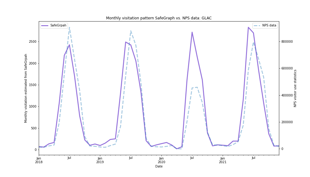
- The first difference correlation between the first difference of Safegraph and NPS monthly series is 0.8316. The first difference correlation is good but Safegraph overestimated the 2020’s visitation.
Glacier NP reported that due to their new visitor registration system they had no way of reporting non-recreational visits to the park for the summer of 2020 which would account for this discrepancy, as SafeGraph records all visitation regardless of recreational or not.
2) Results from __Great Smoky__:
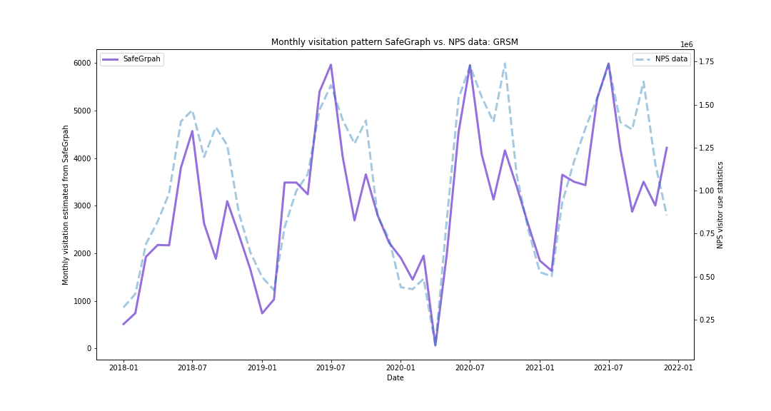
- GRSM first difference correlation: 0.75. GRSM correlation is relatively strong but faces some issues with the Safe Graph data underrepresenting visitation during the fall months.
Due to closures in April 2020 for COVID you can see a severe drop in visitation for that month from both Safe Graph and NPS data. They reopened in May and the numbers increased rapidly from then on before falling back into normal trends.
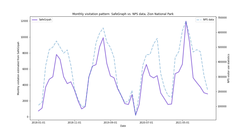
3) Results from __Zion__:
4) Results from __Yellowstone__:
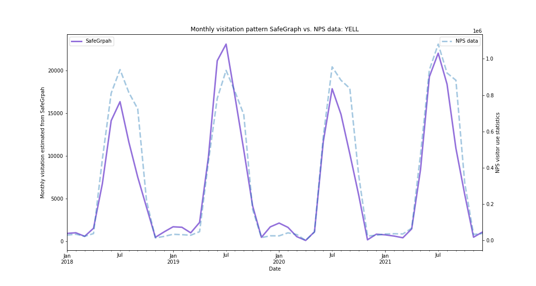
Yellowstone had a very good first-differenced correlation = 0.8816, hence more representative of the visitor population
5) Results from __Acadia__:
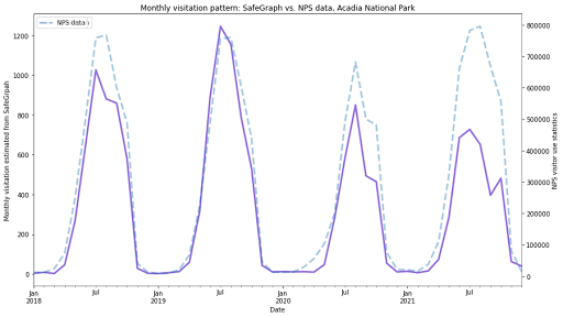
- With a correlation of first differences equal to .93, the Safe Graph and NPS data is shown to be highly correlated for this park.
- The summer of 2021 is the worst fit, with no discernible reason for why the Safegraph data underestimates this time period. This is probably due to a multitude of factors, one being that since July 2021 the Acacia NP visitor calculation system has been non-functional and they have been using estimations. Another explanation could be explained through the dominance of the Jordan Pond House restaurant POI and the various ways that COVID 19 affected restaurant attendance.
- This correlation might be taken with a grain of salt, considering it had the lowest number of POIs. With this in consideration, Yellowstone which has a higher number of POIs, also had a high first difference correlation and might be seen as a more credible example of SafeGraph data validation.
2.2 Comparing the KDE maps across years, we observe that the distribution of visitation derive from Safegraph changed due to multiple reasons.
1) Results from __Glacier__:
The safe graph data of Glacier is somewhat unstable due to the fact that:
- A couple of POIs stopped reporting data in 2020. In total, there are 14 POIs found within the Glacier, but only 11 are reporting data in 2020.
- This sudden drop in the number of “active” POIs can also be observed from the skinny cluster on 2020’s heatmap.
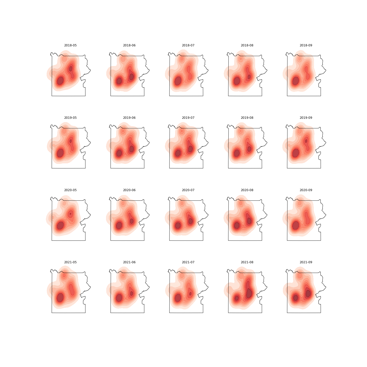
2) Results from __Great Smoky__:

99 POIS is the most abundant, providing more accurate spatial data:
- You can observe the visitors expanding to the southern part of the park in more recent years/months, this trend is also visible in Yellowstone, another park with a large amount of POIs.
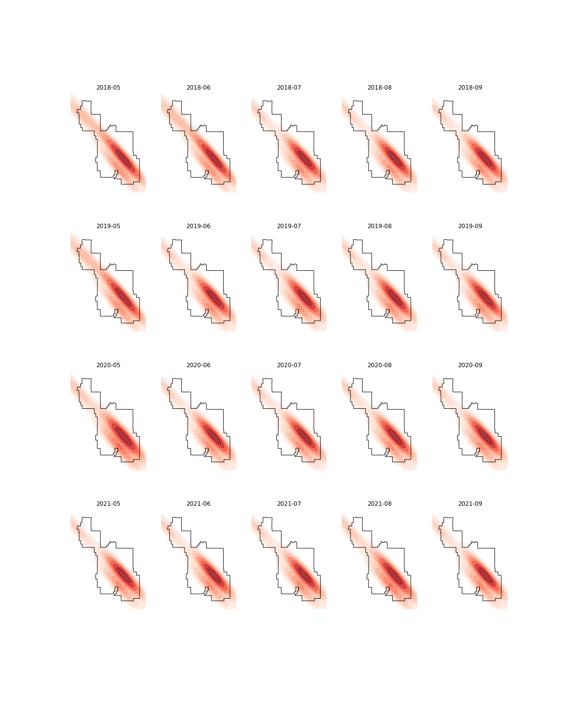
3) Results from __Zion__:
4) Results from __Yellowstone__:
 55 POIS is a robust sample, providing more trustworthy data.
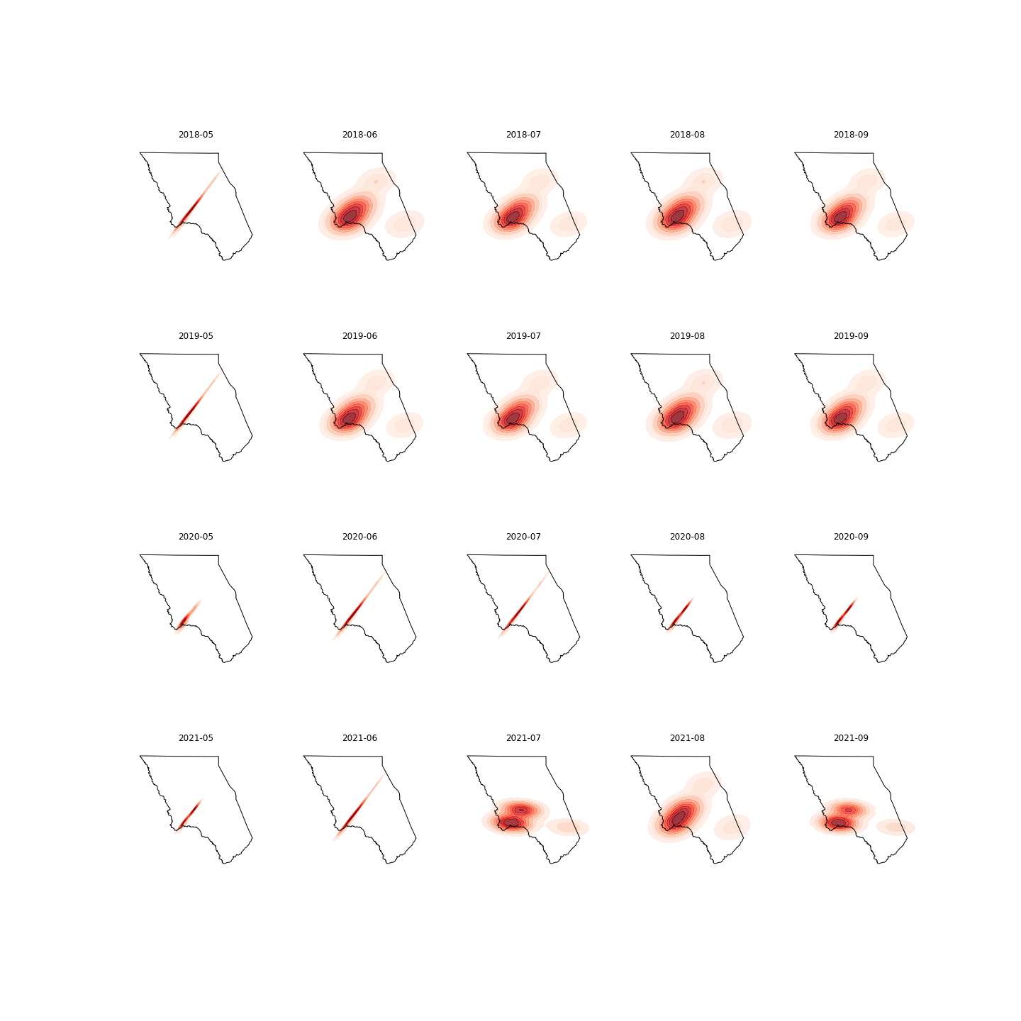
5) Results from __Acadia__:
 Only 10 POIs found within the park. If the number of POI is small, Safegraph data doesn’t seem to capture NPS visitation that well.
3.3 Road network analysis
For Great Smoky NP: Compare the interactive maps of Aug.1 2018 with that of Aug.1 2021. Did we observe an increase/decrease in the congestion in the road network after the pandemic?
- Traffic conditions on Aug 02, 2018: Click map of Aug 02, 2018
- Traffic conditions on Aug 01, 2021: Click map of Aug 01, 2021
Part 2: Code demo, an example of Glacier National Park
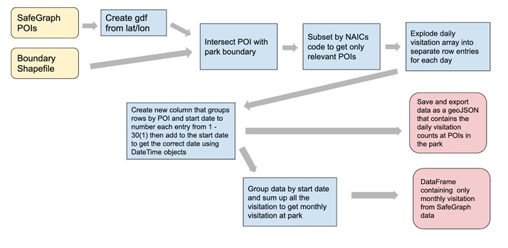
1. Data cleaning (not run)
- Input:
- SafeGraph pattern dataset downloaded at the state level (
MT.csv) - Park boundary (
nps_boundary.shp)
- SafeGraph pattern dataset downloaded at the state level (
- Process: spatial subsetting, geocoding
- Results:
- Daily visiation time series of in-park POIs
- A GeoJSON file that contains these in-park POIs for subsequent analysis
# Load data and convert dataframe to geodataframe using lon and lat columns
boundary = gpd.read_file('../raw_data/nps_boundary/nps_boundary.shp') # boundary shapefile
boundary = boundary.set_index('UNIT_CODE')
df = pd.read_csv('../raw_data/SafeGraph/MT.csv') # safegraph data
gdf = gpd.GeoDataFrame(df,
crs = "EPSG:4269",
geometry = gpd.points_from_xy(df.sg_c__longitude, df.sg_c__latitude))
# Geocode POIs with missing lot-lat info
gdf_na = gdf[gdf['geometry'].is_empty]
gdf_na["address"] = gdf_na['sg_mp__street_address'] + ', ' + gdf_na['sg_mp__city'] + ', ' + gdf_na['sg_mp__region'] + ' ' + gdf_na['sg_mp__postal_code'].astype(int).astype(str)gdf_na['sg_mp__postal_code'].astype(int).astype(str)
na_poi = gdf_na[['placekey', 'address']].drop_duplicates()
geo = geocode(na_poi['address'], provider='nominatim', user_agent = 'autogis_xx')
geo['geometry'].intersects(boundary.at[park, 'geometry']).sum() # check these POIs don't fall within park boundary, so disregard them
# Subset POIs located within the park boundary of Glacier NP
subset_gdf = gdf.loc[gdf['geometry'].intersects(boundary.at['GLAC', 'geometry'])]
subset_gdf = subset_gdf.dropna(subset = ['sg_mp__visits_by_day']) # drop NA in the daily visitation column due to data error
# Explode daily visitation column to multiple rows
subset_gdf.sg_mp__visits_by_day = subset_gdf.sg_mp__visits_by_day.apply(literal_eval) # convert from string to JSON list
subset_gdf = subset_gdf.explode('sg_mp__visits_by_day') # explode it vertically and have each row representing a day
# Create date column to indicate the exact date of year
subset_gdf['n_of_day'] = subset_gdf.groupby(['date_range_start','placekey']).cumcount()
subset_gdf['date_range_start'] = pd.DatetimeIndex(subset_gdf.date_range_start) # convert from string to date
subset_gdf['date'] = pd.DatetimeIndex(subset_gdf.date_range_start) + pd.to_timedelta(subset_gdf['n_of_day'], unit = 'd')
# save a subset of POIs as GeoJSON file.
subset_gdf.to_file('../clean_data/POI_GLAC.geojson', driver = 'GeoJSON')
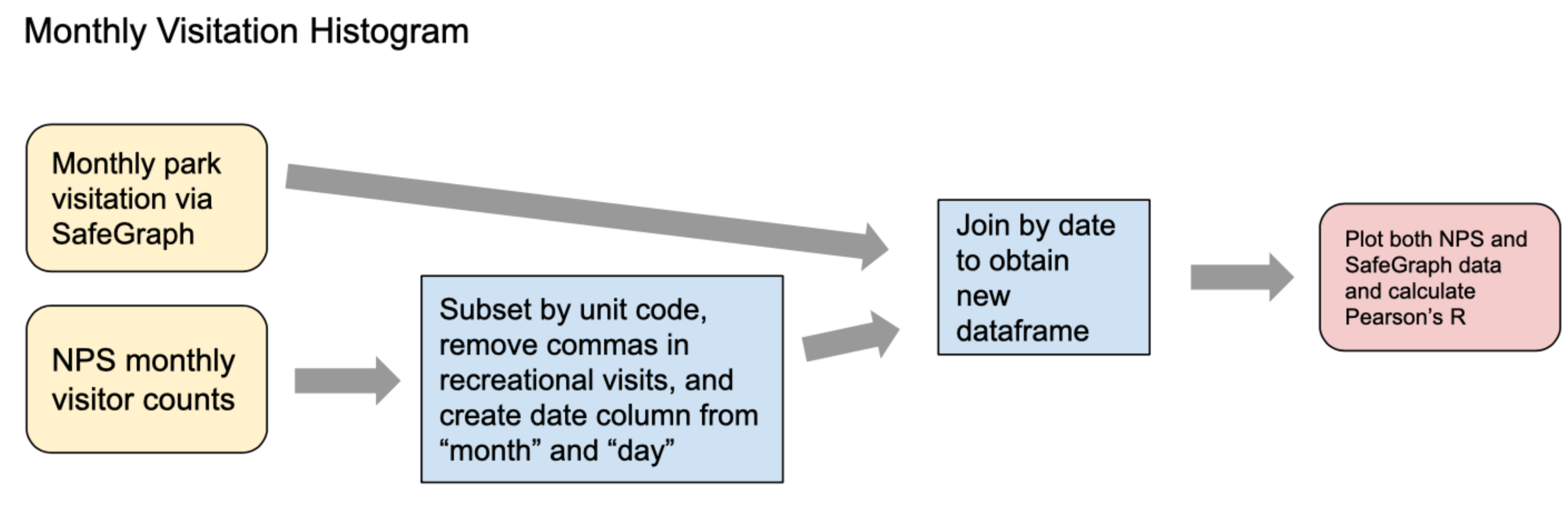
2. Data validation
- Input:
- GeoJSON file that contains POIs found within the Glacier park boundary (
GeoJSON) - NPS monthly visitor counts (
nps_visit_2015_2021.csv)
- GeoJSON file that contains POIs found within the Glacier park boundary (
- Tasks: temporal aggregation, merging
- Results:
- A time series plot comparing two data sources
- A density plot to gauge the spatial dynamics
# !pip install geoplot
import geopandas as gpd
import pandas as pd
from geopandas.tools import geocode
from ast import literal_eval
import matplotlib.pyplot as plt
import geoplot
import osmnx as ox
import networkx as nx
from tqdm import tqdm, trange
Load the cleaned GeoJSON file:
# Load saved GeoJSON
subset_gdf = gpd.read_file('./data/POI_GLAC.geojson')
# load park boundary
boundary = gpd.read_file('./data/nps_boundary.geojson')
boundary = boundary.set_index('UNIT_CODE')
# convert variable to propoer format
subset_gdf['date_range_start'] = pd.DatetimeIndex(subset_gdf.date_range_start) # convert to datetime
subset_gdf['sg_mp__visits_by_day'] = pd.to_numeric(subset_gdf['sg_mp__visits_by_day']) # convert to numeric
subset_gdf.head()
Aggreagate safegraph daily visitaiton to the park-month level: by 'date_range_start'(column for year-month)
park_month = subset_gdf.groupby('date_range_start')['sg_mp__visits_by_day'].sum().to_frame()
Load NPS monthly visitor counts:
nps = pd.read_csv('./data/nps_visit_2015_2021.csv')
nps = nps[nps['UnitCode'] == 'GLAC'] # filter data for Glacier only
nps['RecreationVisits'] = nps['RecreationVisits'].str.replace(",", "").astype(float) # convert to numeric data
# Create a column to indicate year-month
nps['date'] = pd.to_datetime(nps[['Year', 'Month']].assign(DAY = 1))
Merge Safegraph monthly data to NPS visitation:
month_df = nps.set_index('date').join(park_month, how = 'inner') # Inner join by year-month column
month_df['sg_mp__visits_by_day'] = pd.to_numeric(month_df['sg_mp__visits_by_day']) # convert to numeric
month_df.head()
2.1 Time series plot: validate two datasets on the time dimension
f, a = plt.subplots(figsize = (15, 8))
month_df['sg_mp__visits_by_day'].plot(ax = a, color = 'mediumpurple', label = "SafeGrpah", lw = 3)
plt.legend(loc = "upper left")
a2 = a.twinx()
month_df['RecreationVisits'].plot(ax = a2, linestyle = "--", alpha = .4, label = "NPS data", lw = 3)
plt.legend(loc = "upper right")
plt.legend()
a.set(xlabel = "Date",
ylabel = "Monthly visitation estimated from SafeGrpah",
title = f"Monthly visitation pattern SafeGraph vs. NPS data: GLAC")
a2.set(ylabel = "NPS visitor use statistics");

In addition, calculate Pearson correlation between Safegraph and NPS monthly times series:
# calculate correlation
corr = month_df['sg_mp__visits_by_day'].corr(month_df['RecreationVisits'])
# calculate the correlation between first differnced time series
corr_l1 = month_df[['sg_mp__visits_by_day', 'RecreationVisits']].diff().corr().iloc[0, 1]
print(f'''The Pearson correlation between Safegraph and NPS data is {round(corr, 2)}.''')
print(f'''The Pearson correlation between first-differnced Safegraph and NPS data is {round(corr_l1, 2)}.''')
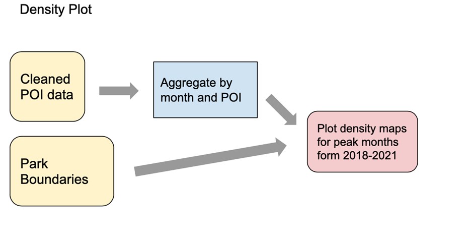
2.2 Density plot: gauge the spatial dynamics of visitation derived from Safegraph over time
Aggregate safegraph daily visitaiton to the POI-month level: by 'placekey'(an indicator for POI) and'date_range_start'(column for month):
poi_month = subset_gdf.groupby(['placekey', 'date_range_start'])['sg_mp__visits_by_day'].sum().to_frame()
Extract geo-coordinates of each POI and merge to the newly created poi_month:
lon_lat = subset_gdf[['placekey', 'geometry']].drop_duplicates().set_index('placekey')
poi_month = poi_month.join(lon_lat, how = 'left').sort_values(by = "date_range_start") # merge & sort by date
# Convert the dataframe to geodataframe:
poi_month_gdf = gpd.GeoDataFrame(poi_month,
crs = "EPSG:4269",
geometry = poi_month.geometry)
For density plot, we focus on peak visitation season (May to Oct). Here we select months to generate the density plot:
temp = poi_month_gdf.reset_index()
temp = temp[temp['date_range_start'].dt.month.isin(range(5,10))]
temp.head()
Density plot of monthly visits to Safegraph POIs overlayed with the Glacier boundary:
proj = geoplot.crs.AlbersEqualArea(central_latitude = boundary[boundary.index == 'GLAC'].centroid.y[0],
central_longitude = boundary[boundary.index == 'GLAC'].centroid.x[0])
months = temp['date_range_start'].unique()
plt.figure(figsize = (20, 20))
for idx, month in enumerate(months):
ax = plt.subplot(4, 5, idx + 1, projection = proj)
geoplot.kdeplot(temp[temp['date_range_start'] == month],
# clip = boundary[boundary.index == 'GLAC'].geometry,
shade = True,
cmap = 'Reds',
#thresh = 0.2,
levels = 10,
alpha = 0.8,
projection = proj,
#cbar = True,
vmin = 0,
#vmax = 309,
ax = ax)
geoplot.polyplot(boundary[boundary.index == 'GLAC'], ax = ax, zorder = 1)
ax.set_title(month.astype('datetime64[M]')) # convert to year-month

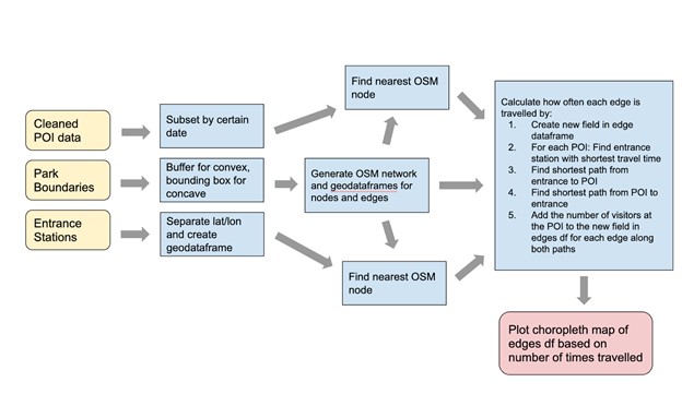
3. Road network analysis
- Input:
- GeoJSON file that contains POIs found within the Glacier park boundary (
GeoJSON) - Park boundary (
nps_boundary.shp) - Geo-locations of park's entrance stations(
entrance_coord.csv)
- GeoJSON file that contains POIs found within the Glacier park boundary (
- Tasks: temporal aggregation, merging
- Results:
- A time series plot comparing two data sources
- A density plot to gauge the spatial dynamics
from IPython.display import Image
from IPython.display import HTML
Load entrance station locations:
entry = pd.read_csv(f'./data/entrance_coord.csv')
# split by "," to create lontitude and latitude columns
lat = []
lon = []
for row in entry['lat_lon']:
lat.append(row.split(',')[0]) # Split the row by comma and append
lon.append(row.split(',')[1])
# Create two new columns from lat and lon
entry['lat'] = lat
entry['lon'] = lon
# convert to geodataframe
entry_gdf = gpd.GeoDataFrame(entry,
crs = "EPSG:4269",
geometry = gpd.points_from_xy(entry.lon, entry.lat))
# filter the entrance stations for Glacier
entry_gdf = entry_gdf[entry_gdf.unitCode == 'GLAC'].reset_index(drop = True)
entry_gdf
(1) For parks with convex shape (Glacier, Yellowstone, Smokies), it's ideal to create a buffer around the park boudary and use this buffer to query osm road network.
# To create buffer, need to first project to UTM (unit: meters)
buff = boundary.loc[['GLAC']].to_crs(epsg = 26912).buffer(8000) # For Glacier: NAD83 / UTM zone 12N
buff = gpd.GeoDataFrame(geometry = gpd.GeoSeries(buff))
# create network from that buffer
G = ox.graph_from_polygon(buff.to_crs(epsg = 4326).geometry[0], network_type = 'drive', simplify = True)
G = ox.project_graph(G, to_crs = 'epsg:4269') # Reproject
ox.plot_graph(G)

(2) For parks with concave shape (Zion and Acadia), better to use the bounding box instead of a buffer.
# # create bounding box based on park boundary
# bound = boundary.loc[[park]].total_bounds
# # Specify the coordinates of four bounds
# north, south, east, west = bound[3], bound[1], bound[2], bound[0]
# # create network from that bounding box
# G = ox.graph_from_bbox(north, south, east, west, network_type = 'drive', simplify = True)
# ox.plot_graph(G)
Convert the OSM road network to GeoPandas GeoDataFrame:
nodes, edges = ox.graph_to_gdfs(G, nodes = True, edges = True, node_geometry = True)
edges.head()
Choose a date that we would like to generate maps for. At the end of the day, we would like to compare the congestion conditions between the same time period of different years, such as the first Friday of August in 2018 vs. 2020.
day = '2018-08-02'
# change variable type
subset_gdf['date'] = pd.DatetimeIndex(subset_gdf.date) # convert string to datetime
subset_gdf['sg_mp__visits_by_day'] = pd.to_numeric(subset_gdf['sg_mp__visits_by_day']) # convert to numeric
# filter data by the chosen date
poi_gdf = subset_gdf.loc[subset_gdf['date'] == day,
['placekey', 'date', 'sg_c__location_name', 'geometry', 'sg_mp__visits_by_day']].reset_index(drop = True)
poi_gdf
Plot entrance stations and POIs together with the park road network:
m = edges[edges.highway == 'secondary'].explore()
poi_gdf.drop(['date'], axis = 1).explore(m = m,
column = 'sg_mp__visits_by_day',
cmap = "RdBu_r",
marker_type = 'circle',
marker_kwds = {'radius': 1000,
'fill': True
}
) # POIs
entry_gdf.explore(m = m,
marker_type = 'marker'
) # entrances
# A function helps you to find the nearest OSM node from a given GeoDataFrame (cr. Dr.Park)
def find_nearest_osm(network, gdf):
"""
# This function helps you to find the nearest OSM node from a given GeoDataFrame
# If geom type is point, it will take it without modification, but
# IF geom type is polygon or multipolygon, it will take its centroid to calculate the nearest element.
Input:
- network (NetworkX MultiDiGraph): Network Dataset obtained from OSMnx
- gdf (GeoDataFrame): stores locations in its `geometry` column
Output:
- gdf (GeoDataFrame): will have `nearest_osm` column, which describes the nearest OSM node
that was computed based on its geometry column
"""
for idx, row in tqdm(gdf.iterrows(), total=gdf.shape[0]):
if row.geometry.geom_type == 'Point':
nearest_osm = ox.distance.nearest_nodes(network,
X=row.geometry.x,
Y=row.geometry.y
)
elif row.geometry.geom_type == 'Polygon' or row.geometry.geom_type == 'MultiPolygon':
nearest_osm = ox.distance.nearest_nodes(network,
X=row.geometry.centroid.x,
Y=row.geometry.centroid.y
)
else:
print(row.geometry.geom_type)
continue
gdf.at[idx, 'nearest_osm'] = nearest_osm
return gdf
Find the nearest OSM node for each POI within the park:
poi_gdf = find_nearest_osm(G, poi_gdf)
poi_gdf
Similarly, find the nearest OSM node for each entrance station:
entry_gdf = find_nearest_osm(G, entry_gdf)
entry_gdf
Calculate the times that each edges has been passed through by visitors on that day:
edges['travel_times'] = 0
for idx_p, row_p in poi_gdf.iterrows(): # loop for each POI
length = []
for idx_e, row_e in entry_gdf.iterrows(): # Loop for each entrance station
# Calculate the shortest driving distance from every entrance station to a specific POI
temp_length = nx.shortest_path_length(G = G,
source = row_e['nearest_osm'],
target = row_p['nearest_osm'],
weight = 'length',
method = 'dijkstra'
)
length.append(temp_length)
# Find the nearest entrance station from that POI
val, idx = min((val, idx) for (idx, val) in enumerate(length)) # get the position in the list with smallest number
# Get shortest paths from the nearest entrances to that POI. Visitors are assumed to take this route to enter the park.
start_route = nx.shortest_path(G = G,
source = entry_gdf.loc[idx, 'nearest_osm'],
target = row_p['nearest_osm'],
weight = 'length',
method = 'dijkstra'
)
for i in range(len(start_route) - 1):
cum_sum = edges.loc[(edges.index.get_level_values('u') == start_route[i]) & (edges.index.get_level_values('v') == start_route[i+1]), 'travel_times'] + row_p['sg_mp__visits_by_day']
edges.loc[(edges.index.get_level_values('u') == start_route[i]) & (edges.index.get_level_values('v') == start_route[i+1]), 'travel_times'] = cum_sum
# Get shortest paths from the that POI to the nearest entrances. Visitors are assumed to take this route to exit the park.
back_route = nx.shortest_path(G = G,
source = row_p['nearest_osm'],
target = entry_gdf.loc[idx, 'nearest_osm'],
weight = 'length',
method = 'dijkstra'
)
for i in range(len(back_route) - 1):
cum_sum = edges.loc[(edges.index.get_level_values('u') == back_route[i]) & (edges.index.get_level_values('v') == back_route[i+1]), 'travel_times'] + row_p['sg_mp__visits_by_day']
edges.loc[(edges.index.get_level_values('u') == back_route[i]) & (edges.index.get_level_values('v') == back_route[i+1]), 'travel_times'] = cum_sum
# A preview of the summary statistiscs
edges.travel_times.describe()
Now we are ready to visualize the congestion conditions: color code edges using Red/Yellow/Green palettes, based on the number of visitors who may pass through each road segment.
m = edges.explore(tiles = 'Stamen Terrain',
column = 'travel_times',
cmap = 'RdYlGn_r',
scheme = 'NaturalBreaks',
k = 5,
vmin = 0,
highlight = True,
tooltip = ['name', 'travel_times'], # displayed upon hovering
popup = True, # all columns displayed upon clicking
legend_kwds = {
'caption': 'Congestion',
'scale': False,
'colorbar': False
}
)
entry_gdf.explore(m = m,
marker_type = 'marker',
tooltip = ['entrance']
) # entrances